This post is the third and last part of the series Neural Network Demystified. If you haven’t read the first two parts please check Neural Network Demystified Part l – Building Blocks and Activation Functions and Neural Network Demystified Part lI – Deep Neural Network first.
Training a Neural Network
Neural networks are used for three main categories of learning, namely as supervised, unsupervised and reinforcement learning. Training of a neural network involves the combination of several individual algorithms and helper components like a base architecture, optimisation algorithm called gradient descent, convolution, pooling, softmax classifier etc. In this article, three of the most important components are explained.
-
Loss Function
The loss function, also called a cost function, is a measure of quantifying the capacity of a network to approximate the true function that produces the desired output from given data. In supervised learning, desired output is the ground truth labels or classes \( \hat{y} \) of each sample in the dataset. In a single forward pass, the network takes as inputs the weights, biases and examples from the training set and predicts the labels \( \hat{y} \) for each sample. The difference between the predicted labels and the ground truth labels are calculated which is the total loss of the network. Although there are many loss functions that exist, all of them essentially penalize on the difference or error between the predicted \( \hat{y} \) for a given sample and its actual label y. Mean squared error or MSE is a commonly used loss function. For \( m \) number of samples in the training set, the equation for calculating total loss over weight parameters, \( J(w_{1},…w_{n}) \) using MSE is shown in Equation 1.
\[ Loss(y,\hat{y}) = J(w_{1},…w_{n}) = \frac{1}{m}\sum_{i=1}^{m}\left ( y_{i}-\hat{y_{i}} \right )^{2}\;\;\;(1) \]
-
Gradient Descent
The purpose of training a neural net is to minimize the loss by adjusting the parameters, like weights, biases etc. The smaller the loss, the more accurately the true function is approximated. Gradient descent algorithms are the most commonly used methods for loss function optimization. At the beginning of the training, network parameters are randomly initialized. Therefore, the loss is very high. Gradient descent algorithms calculate the first order derivative of each of the parameters with respect to the loss function and directs in which direction the parameter values have to be adjusted in order to reduce the loss. Eventually, it finds the global minimum of the loss function curve which is the point at which the loss is minimum. All model parameters including weights are defined as θ. Therefore, for each \( \theta_{j} \), gradient descent algorithms find the derivative of each \( \theta_{j} \) for each input vector \( X_{0} \) to \( X_{n} \) with respect to total loss \( J(\theta_{j0},…\theta_{jn}) \) and update each parameter using Equation 2.
\[ \theta_{j} := \theta_{j} \;-\; \alpha \frac{\partial }{\partial \theta_{j}} J(\theta_{j0},…\theta_{jn})\;\;\;(2) \]
Here, α is the learning rate that defines the step size in the direction the parameters are adjusted to. The algorithm iteratively performs this operation until either the global minimum is reached or the model converges.
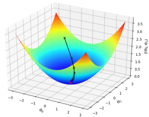
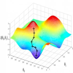
The feature space of the loss function can be convex or even highly non-convex with tens of millions of parameters depending on model complexity. Fig. 1 and Fig. 2 show examples of gradient descent in both convex and non-convex loss surface having only two parameters \( \theta_{0} \) and \( \theta_{1} \). The black line shows the gradient started from an initial point flowing all the way down to the global minimum on convex and local minimum on non-convex surface.
-
Backpropagation
Calculating the derivatives of millions of parameters with respect to total loss and find the optimal point in a high-dimensional convex or non-convex surface is analogous to finding a needle in a haystack. Accomplishment of this task using the naive approach is extremely unfeasible. That’s where backpropagation comes to the rescue. Back- propagation is a fast way of calculating all the parameter gradients in a single forward and backward pass through the network rather than having to do one single pass for every single parameter. It utilizes the chain rule of partial derivatives to compute gradients on a continuously differentiable multivariate function in a neural network. The chain rule enables gradient descent algorithms to decompose a parameter derivative as a product of its individual functional components. Use of backpropagation allows a backward pass take roughly the same amount of computation as a forward pass and makes doing gradient descent on deep neural networks a feasible problem by speeding up the training dramatically.
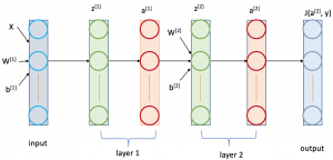
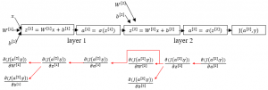
Fig. 3(b) illustrates backpropagation in action in a neural network with two hidden layers layer 1 and layer 2 as shown in Fig. 3(a). After a forward pass (shown with black arrow) the loss function \( J(a^{[2]},y) \)is evaluated. Then, in the backward pass (shown in red arrow), the partial derivative of each of the four parameters \( W^{[1]} \), \( b^{[1]} \), \( W^{[2]} \) and \( b^{[2]} \) with respect to \( J(a^{[2]},y) \) is calculated using chain rule. As example, to calculate the partial derivative of \( W^{[1]} \), we have to first partially derive \( z^{[1]} \) (the weighted sum function in layer 1) with respect to \( J(a^{[2]},y) \) as \( \frac{\partial ( J(a^{[2]},y) )}{\partial z^{[1]}} \). Again, in order to find \( \frac{\partial ( J(a^{[2]},y) )}{\partial z^{[1]}} \), \( \frac{\partial ( J(a^{[2]},y) )}{\partial a^{[1]}} \) has to be calculated where \( a^{[1]} \) is the layer 1 activation function. Consequently, the derivative of \( a^{[1]} \) comes from the derivative of functions \( z^{[1]} \) and \( a^{[2]} \) in layer 2. In this way, backpropagation propagates the total loss backward all the way down to each parameters and adjust them accordingly using gradient descent. Therefore, it gives a detailed insight into how changing the weights and biases changes the overall behaviour of the network a.k.a the change in total network loss.
The above three components combined are run lot many times or iterations during the training phase. After each iteration the global loss of a neural network is reduced from the previous iteration, indicating that the network is being trained better and better.
This was the last part of the series Neural Network Demystified. I hope you have found this article and the series useful. Please feel free to comment below about any questions, concerns or doubts you have. Also, your feedback on how to improve this blog and its contents will be highly appreciated. I would really appreciate you could cite this website should you like to reproduce or distribute this article in whole or part in any form.
You can learn of new articles and scripts published on this site by subscribing to this RSS feed.
Actually when someone doesn’t be aware of afterward its up to other viewers
that they will help, so here it occurs.
Thanks for a marvelous posting! I certainly enjoyed reading
it, you’re a great author. I will make sure to bookmark your blog
and will often come back someday. I want to encourage one to continue your great job, have a nice evening!
Hi Royal CBD, thanks for your kind words! Glad that it helped you.
Hello there, just became alert to your blog through Google, and found that it’s
really informative. I am going to watch out for brussels.
I will appreciate if you continue this in future.
A lot of people will be benefited from your writing.
Cheers!
P.S. If you have a minute, would love your feedback on my new website re-design. You can find it
by searching for “royal cbd” – no sweat if you can’t.
Keep up the good work!
Hi Justin, thanks for your kind words! Glad that it helped you. I will check your website 🙂
Long time supporter, and thought I’d drop a comment.
Your wordpress site is very sleek – hope you don’t mind
me asking what theme you’re using? (and don’t mind if I steal it?
:P)
I just launched my site –also built in wordpress like yours– but
the theme slows (!) the site down quite a bit.
In case you have a minute, you can find it by searching for “royal cbd” on Google (would appreciate any feedback) – it’s still in the works.
Keep up the good work– and hope you all take care of yourself during the coronavirus scare!
I don’t typically comment on posts, but as a long time reader I thought
I’d drop in and wish you all the best during these troubling times.
From all of us at Royal CBD, I hope you stay well with the COVID19 pandemic progressing at an alarming rate.
Justin Hamilton
Royal CBD