This post is the second part of the series Neural Network Demystified. If you haven’t read the first part please check Neural Network Demystified Part I – Building Blocks and Activation Functions first.
Arti ficial Neural Networks
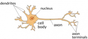
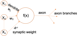
Artifi cial Neural Networks (ANNs) are motivated by the nervous system of the human brain where approximately 86 billion neurons are interconnected with \( 10^{14} \) to \( 10^{15} \) synapses. In human nervous system, each neuron receives input signals from its dendrites and produces output signal along its axon. Comparatively, ANNs are a way smaller and simplifi ed computing model of the nervous system with tens to as many as thousands of neurons interconnected as processing elements, which process information by their dynamic state response triggered by external inputs (i.e. user given data). As seen in Fig. 1, just like a biological neuron has dendrites to receive signals, a cell body to process them, and an axon to send signals out to other neurons through axon branches, the arti ficial neuron has a number of input channels, a processing stage called f(x), and one output analogous to axon branches that can fan out to multiple other arti ficial neurons. ANNs are comprised of stacks of layers, where each layer contains a pre-de fined number of neurons just like the one in the fi gure. Neurons from each layer are connected by edges which are similar to synapses. Axons are analogous to the output obtained from a single layer.
Any shallow neural network has at least three layers, namely as an input layer, hidden layer(s) and an output layer. Hidden layers are intermediate layers between input and output layer. In Fig. 2, the network has 7 neurons altogether. These neurons are stacked in 3 fully connected layers, that is each neuron from one layer is connected to each neuron from the following layer. The number of layers in the network, the number of neurons in each layer, how they are connected (as example, fully-connected or locally connected) – all these are usually pre-defi ned while designing the network architecture. First layer, consisting of 3 neurons, is the input layer where these neurons do not participate in any kind of calculation, rather they just propagate the input to the next hidden layer with their associated weights and bias. For simplicity, in this network the bias term is omitted. The hidden layer calculates the weighted sum from each neuron and passes the result as a 3 x 3 matrix to the ReLU activation function. The output of ReLU is used as input to the output layer. In the output layer, sigmoid activation function is used to transform the resultant matrix into a categorical or numerical value which is the fi nal output of the network.
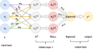
In Fig. 2, \( h_{1}^{[1]} \), \( h_{2}^{[1]} \) and \( h_{3}^{[1]} \) are the neurons of hidden layer 1. From the network, they are calculated individually from the weighted sum of \( x_{1} \), \( x_{2} \) and \( x_{3} \) as following,
\( h_{1}^{[1]} = w_{1}\cdot x_{1}+w_{4}\cdot x_{2}+w_{7}\cdot x_{3} \)
\( h_{2}^{[1]} = w_{2}\cdot x_{1}+w_{5}\cdot x_{2}+w_{8}\cdot x_{3} \)
\( h_{3}^{[1]} = w_{3}\cdot x_{1}+w_{6}\cdot x_{2}+w_{9}\cdot x_{3} \)
Now \( h_{1}^{[1]} \) , \( h_{2}^{[1]} \) and \( h_{3}^{[1]} \) are passed to corresponding ReLU activation function \( A_{1}^{[1]} \) , \( A_{2}^{[1]} \) and \( A_{3}^{[1]} \) for non-linear transformation. The weighed sum of the activations generates the final output \( \hat{y} \). \( w_{10} \), \( w_{11} \) and \( w_{12} \) are weights associated to \( A_{1}^{[1]} \) , \( A_{2}^{[1]} \) and \( A_{3}^{[1]} \) respectively. Therefore, the function for calculating \( \hat{y} \) is defined in the following equation,
\( \hat{y} \) = \( f\left ( x_{1},x_{2}, x_{3} \right ) \) = \( Sigmoid(w_{10}\times ReLU({h_{1}}^{[1]}) + w_{11}\times ReLU({h_{2}}^{[1]}) + w_{12}\times ReLU({h_{3}}^{[1]})) \)
Deep Neural Network
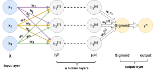
Deep neural networks (DNNs) are basically ANNs with many hidden layers ranges from 3 to 152 (ResNet). The more layers stacked up in between the input and output layer, the deeper the network is considered. The deeper the network, the more complex representation from the data can be learned. The hidden layers learn data representation in hierarchical order, which means that the output of a hidden layer is passed as input to its next consecutive hidden layer and so on.
Many recent breakthrough outcomes are obtained by using very deep models. However, stacking up layers after layers does not always guarantee better model accuracy. In Deep residual learning for image recognition (CVPR 2016), authors have reported that with network depth increasing, the accuracy gets saturated after one point. Also, deeper models require to compute larger number of parameters which makes them computationally expensive and slower. Fig. 3 shows a deep neural network with \( n \) hidden layers.
Next part is Neural Network Demystified Part III – Gradient Descent and Backpropagation.
I hope you have found this article useful. Please feel free to comment below about any questions, concerns or doubts you have. Also, your feedback on how to improve this blog and its contents will be highly appreciated. I would really appreciate you could cite this website should you like to reproduce or distribute this article in whole or part in any form.
You can learn of new articles and scripts published on this site by subscribing to this RSS feed.