Building Blocks of a Neural Network
Although the original intention of designing a neural network was to simulate the human brain system to solve general learning problems in a principled way, in practice neural network algorithms work in much simpler way than a human brain. Current neural networks can be compared to statistical models having the higher level purpose of mapping inputs to their corresponding outputs. By the means of lots of complex matrix computations going on under the hood, they try to find correlations by approximating an unknown function f(x) = y between any input x and any output y. In the process of learning, they drive to discover the most accurate function f which is also the best approximation of transforming x into y. These networks can be both linear or non-linear. Non-linear networks can approximate any function with an arbitrary amount of error. For this reason, they are also called “universal approximator”. In this tutorial, let us learn about the building blocks of a non-linear shallow neural network followed by the architecture of a standard deep neural network.
- A Neuron
An artifi cial neuron (derived from the basic computational unit of the brain called neuron), also referred to as a perceptron is a mathematical function that takes one or more inputs and returns their weighted sum as output. Weighted sum is passed through an activation function to transform the otherwise linear function to a non-linear function. This is the reason why neural networks perform well in deriving very complex non-linear functions. Basically, weights are values associated with each input and are parameters to be learned by the network from input data in order to accurately map them to desired output.
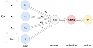
In Fig. 1, input \( X \) is a vector containing three elements \( x_{1} \), \( x_{2} \) and \( x_{3} \). Each element have weights \( w_{1} \), \( w_{2} \) and \( w_{3} \) associated to them respectively. In addition to weights, there is also a bias term \( b \) which helps the function better fi t the data. The neuron \( f(x) \) calculates the weighted sum using Equation 1. \( f(x) \) is also de fined by \( z \) interchangeably.
\[ f(x) = z = w_{1}\cdot x_{1} + w_{2}\cdot x_{2} + w_{3}\cdot x_{3} + b \;\;\;(1) \]
The resultant output is then passed to an activation function A(f(x)) which returns the final output of the neuron.
- Activation Function
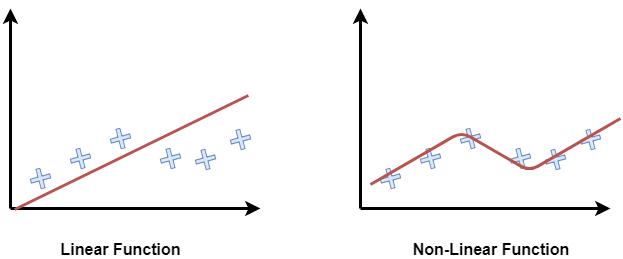
An activation function is a function applied on a neuron to instill some kind of non-linear properties in the network. A relationship is considered as linear if a change in a variable initiates a constant change in the consecutive latter variables. On the other hand, a non-linear relationship between variables is established when a change in one variable does not necessarily ignites a chain of constant changes in the consecutive latter variables, although they can still impact each other in an unpredictable or irregular manner. Without the injection of some non-linearity, a large chain of linear algebraic equation will eventually collapse into a single equation after simplification. Therefore, the significant capacity of the neural network to approximate any convex and non-convex function is directly the result of the non-linear activation functions. In a small visual example in Fig. 2, we can see that when data points make non-linear patterns, a linear line can not t them accurately, thus it misses some data points. However, a non-linear function captures the difficult pattern efficiently and fi ts all data points.
Every activation function takes the output of f(x) as a vector as input and performs a pre-de fined element-wise operation on it. Among many activation functions, three of them are most commonly used.
Sigmoid
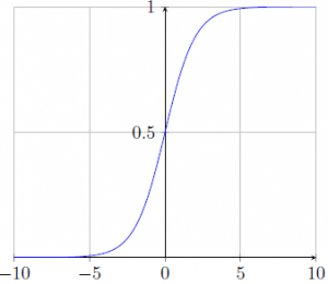
The sigmoid non-linearity function has the following mathematical form,
\[ sigmoid(f(x)) = \frac{\mathrm{1} }{\mathrm{1} + e^{-f(x) }}\;\;(2) \]
It takes a real value as input and squashes it between 0 and 1 so that the range does not become too large. However, for large values of neuron activation at either of the positive or negative x-axis, the network gets saturated and the gradients at these regions get very close to zero (i.e. no signifi cant weight update in these regions), causing “vanishing gradient” problem. Fig. 3 shows the sigmoid function graph that converges in the positive and negative domain as values get bigger.
Hyperbolic Tangent
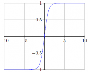
The hyperbolic tangent or tanh non-linearity function has the following mathematical form,
\[ tanh(f(x)) = \frac{e^{f(x)}-e^{-f(x)}}{e^{f(x)}+e^{-f(x)}}\;\;(3) \]
It takes a real value as input and squashes it between -1 and 1. However, it suffers from the “vanishing gradient” problem in the positive and negative domain like sigmoid function for similar reason. Fig. 4 shows the graph for hyperbolic tangent function.
Recti ed Linear Unit (ReLU)
The ReLU has the following mathematical form,
\[ ReLU(f(x)) = max(0,f(x))\;\;(4) \]
ReLU has gained huge popularity as an activation function due to its edge over sigmoid and tanh in couple of ways. It takes a real value as input and squashes it between 0 and +infi nity. Because it does not saturate in the positive domain, it avoids the vanishing gradient problem. As a result, it also accelerates the convergence of stochastic gradient descent. Another big advantage of ReLU is that it involves computationally cheaper operations compared to the expensive exponentials in sigmoid and tanh. However, ReLU saturates in the negative domain which allows it to disregard all the negative values. Thus it may not be suitable to capture patterns in all different datasets and architectures. One solution to this problem is LeakyReLU.
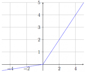
Instead of zeroing out the negative activation, LeakyReLU applies a small negative slope of 0.01 or so. Therefore, LeakyReLU has the following mathematical form, where α is the slope.
\[ LeakyReLU\left ( f\left(x \right ) \right ) = \left\{\begin{matrix} max(0, x)\;\;for\;\;f(x) > 0\\ αx\;\; for\;\;f(x)<0 \end{matrix}\right. \;\;(5) \]
Fig. 5 shows ReLU graph where slope keeps increasing only in the positive domain.
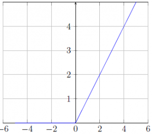
Fig. 6 shows LeakyReLU graph where slope keeps increasing in the positive domain but also allows gradients to flow by a restricted amount in the negative domain. Here, α is 0.1.
Next part is Neural Network Demystified Part ll – Deep Neural Network.
I hope you have found this article useful. Please feel free to comment below about any questions, concerns or doubts you have. Also, your feedback on how to improve this blog and its contents will be highly appreciated. I would really appreciate you could cite this website should you like to reproduce or distribute this article in whole or part in any form.
You can learn of new articles and scripts published on this site by subscribing to this RSS feed.