The current frameworks for object detection task can be categorized into two main types. One category of frameworks uses a two-step pipeline – first it generates region proposals using improved algorithms other than sliding windows, then passes the regions to CNN and SVM for feature extraction followed by classification and localization. The other category unifies the region proposal generation and classification and regression task as one multi-task learning problem. The two-step pipeline methods mainly include R-CNN, Fast R-CNN, Faster R-CNN, R-FCN, FPN, SPP-net etc. The unified methods include Multibox, YOLO, YOLOv2, SSD, DSSD, DSOD etc.
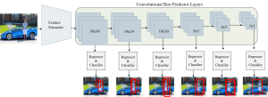
SSD is a one-step framework that learns to map a classification-and-regression problem directly from raw image pixels to bounding box coordinates and class probabilities, in single global steps, thus the name “single shot”. Fig. 1 illustrates the architecture of SSD. It incorporates a Deep Convolutional Neural Network as the base feature extractor similar to Faster R-CNN. However, the fully-connected layers from the extractor is discarded and replaced by a set of auxiliary convolutional layers as shown in blue. These auxiliary layers are responsible for extracting features at multiple scales and progressively decrease the size of the input at each subsequent layer. Instead of generating anchor boxes at each feature map separately like in Faster R-CNN, SSD generates anchor boxes directly on the multi-scale feature maps coming from the base CNN.
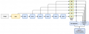
In SSD (ECCV 2016), authors have used six auxiliary layers for producing feature maps of size 8 × 8, 6 × 6, 4 × 4, 3 × 3, 2 × 2 and 1 × 1 respectively. Due to multiple scaling, generated anchor boxes better cover all the diverse shapes of objects including very small objects and very large ones. Features extracted by each region proposal or anchor from each feature map is simultaneously passed to a box regressor and a classifier. Finally, the network outputs coordinate offsets of predictions relative to anchor boxes, objectness score (here confidence score) of each predicted boxes and probabilities of an object inside a predicted box being each of the \( C \) classes. For instance, for feature maps of size \( f = m \times n \), \( b \) anchors per cell in each of the feature maps and \( C \) total classes, SSD will output total \( f \times b \times (4 + c) \)values for each of the six feature maps. Anchors boxes are generated with different aspect ratios and scales similar to Faster R-CNN, however, due to applying them on multiple scaled feature maps objects with more variety of sizes and scales are detected more accurately.
Integrating with some pre and post-processing algorithms like non-maximum suppression and hard negative mining, data augmentation and a larger number of care- fully chosen anchor boxes, SSD significantly outperforms the Faster R-CNN in terms of accuracy on standard PASCAL VOC and COCO object detection dataset, while being three times faster.
As mentioned earlier, SSD framework is a single feed-forward convolutional neural network which performs both object localization and classification in a single forward pass. However, the whole network is composed of six major parts or algorithms and each of them plays crucial role in providing the final output.
- Base Network for Feature Extraction
-
Convolutional Box Predictor
-
Priors generation
-
Matching priors to ground-truth boxes
-
Hard Negative Mining
-
Post-processing – Non-maximum suppression
-
Base Network for Feature Extraction
SSD architecture is based on a deep CNN which works as the feature extractor. Deep CNNs has showed high performance in image classification on many benchmark datasets, which indicates that the features learned by these networks can be very useful in performing other more sophisticated computer vision tasks like object detection as well. In case of real-time inference, MobileNet is a widely used Deep CNN which is at least 10 times faster than its contemporary regular deep CNNs like VGGNet-16, when run in both GPU and CPU.
In MobileNet model, each standard convolutional layer is replaced by two separate layers called a depthwise convolution followed by a pointwise convolution, combinedly called as depthwise separable convolution. A standard convolution layer both filters and combines inputs, no matter how many channels it has, into a new set of single channel output pixels in one step. Whereas the depthwise separable convolution splits this process into two layers, a separate layer for filtering independently on each channel and a separate layer for combining the filtered channels into a single output channel. This factorization has the effect of drastically reducing computation and model size, therefore resulting in a very fast model for real-time performance.
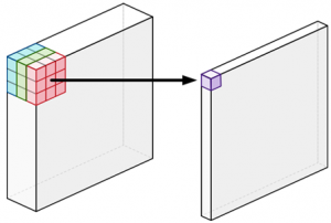
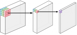
(a) regular convolution (b) depthwise separable convolution
Fig 2. Regular VS depthwise separable convolution (Source)
In Fig. 2(a), regular convolution with 3 × 3 filters on a 3-channel input generates an output of a single channel image pixel in a single go. On the other hand, depthwise separable convolution in Fig. 2(b) at first applies 3 × 3 filters on each of the three channels separately, generating output image that also has 3 channels where each channel gets its own set of weights. In the next step, pointwise convolution is applied which is same as a regular convolution but with a 1 × 1 kernel. Pointwise convolution simply adds up all the output channels of the depthwise convolution as a weighted sum in order to create new features.
Although, the end result of both regular and depthwise separable convolution is similar, a regular convolution has perform much more mathematical computation to obtain the result and needs to learn more weights compared to the latter one. For instance, the number of computation required to perform convolution with 32 3 × 3 filters on a 16-channels input using regular convolution is following,
\[ 16 × 32 × 3 × 3 = 4608 \]
Whereas the number of computation required by depthwise separable convolution is following (7 times faster),
\[ 16 × 3 × 3 + 16 × 32 × 1 × 1 = 656 \]
The original MobileNet architecture uses one regular convolutional layer in the first layer and 13 consecutive depthwise convolution layers each followed by a point-wise separable layer. Batch Normalization (BN) and ReLU activation function are applied after each convolution. After the convolutional layers, there is an Average Pooling layer of kernel 1 × 1 followed by a Fully-connected layer linked to a softmax classifier for classification. Complete architecture of MobileNet is described in the original paper.
-
Convolutional Box Predictor
For object detection task, original base extractor is extended to a larger network by removing and adding some successive layers. From the MobileNet architecture, the last fully-connected layer is discarded and a set of auxiliary convolutional layers are added which are called convolutional box predictor layers. These layers produce multiple feature maps of sizes 19 × 19, 10 × 10, 5 × 5, 3 × 3 and 1 × 1 in successive order which are stacked after the feature map coming from the last convolutional layer of MobileNet of size 38 × 38. All six auxiliary layers extract features from images at multiple scales and progressively decrease the size of the input scan to each subsequent layer. Performing convolution on multiple scales enables detecting objects of various sizes. As example, feature maps of size 19 × 19 performs better in detecting small objects whereas 3 × 3 performs better for larger objects. Each of the box predictor layers is connected to two heads, one regressor to predict bounding boxes and one sigmoid classifier to classify each of the detected boxes. Let’s consider an input image as shown in Fig. 3. The image has three classes of objects, namely as “person”, “car” and “vase”.
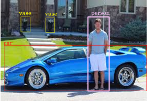
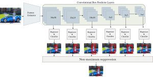
Fig. 4 shows the SSD architecture that consists of base feature extractor and auxiliary predictor layers. Each layer predicts some bounding boxes for the class person. Eventually predictions from all the layers are accumulated in the post-processing layer which provides the final prediction for person as the output. The same procedure follows for each of the classes present in the input image.
-
Priors Generation
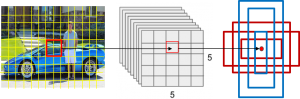
Priors or anchor generation is one of the most important tasks that can significantly affect the overall model performance. Priors are a collection of pre-defined boxes overlaid on the input scan as well as the predictor feature maps at different spatial locations, scales and aspect ratios that act as reference points for the model to predict the ground truth boxes. Ground truth boxes are the boxes that are annotated by human while labeling the dataset. Prior boxes are really important because they provide a strong starting point for the bounding box regression algorithm to predict the ground truth boxes as opposed to starting predictions with completely random coordinates. Each feature map is divided into number of grids and each grid is associated to a set of priors or default bounding boxes of different dimensions and aspect ratios. Each of the priors predict exactly one bounding box. In the following example, there are priors of six aspect ratios for each grid cell in each of the six feature maps. As shown in Fig. 5, each grid cell of a 5 × 5 feature map have six priors which mostly matches with the classes or objects we want to detect. As example, red priors are most likely to capture car whereas blue priors are there to detect person and vase of both smaller and larger sizes. Also, feature maps represent the dominant features of the images at different scales, therefore generating priors on multiple scale feature maps increase the likelihood of any object of any size to be eventually detected, localized and appropriately classified.
-
Matching Priors to Ground-truth Boxes
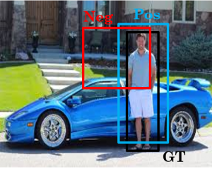
Next, each ground truth box is matched to priors having the biggest Jaccard Index or Intersection over Union (IoU). In addition, unassigned priors having IoU greater than a threshold are also matched to ground truth boxes, usually the threshold is 0.5. At this point, all the matched priors are called positive training examples and rest are considered as negative examples. In Fig. 6, blue prior is a positive example since it has greater IoU with the ground truth box of person showed in black and red prior is a negative example because it does not have IoU greater than 0.5 with any of the ground truth boxes.
-
Hard Negative Mining
Among a large number of priors, only a few will be matched as positive samples and rest of the large number of priors will be left out as negatives. From the training point of view, there will be a class imbalance between positive and negative samples which may make the training set biased towards negatives. To avoid this, some of the negative examples are randomly sampled from the negative pool in such a way so that the training set have a negative to positive ratio of 3:1. This process is called hard negative mining. The reason why it is required to keep negative samples is because the network also needs to learn and be explicitly told about the features that lead to incorrect detection.
-
Post-processing – Non-maximum Suppression
At the prediction stage while both training and inference, every prior will have a set of bounding boxes and labels. As a result, there will be multiple predictions for the same object. Non-maximum suppression algorithm is used to filter out duplicate and redundant predictions and keep the top K most accurate predictions. It sorts the predictions by their confidence score for each class. Then it picks predictions from the top and removes all the other predictions that have IoU greater than 0.5 with the picked one. In this way, it ends up with having maximum one hundred top predictions per class. This ensures that only the most likely predictions are kept by the model, while the more noisier ones are discarded. Fig. 7 shows complete SSD architecture with the non-maximum suppression layer which filters out all the less accurate predictions and generating the one as output with the highest confidence score.
Now that we know about all the individual components, it is time for training this whole framework. As mentioned earlier, because it is a one-step feed-forward end-to-end learning model, all of these components are trained simultaneously at each single iteration. The training process is explained in the next part Training Single Shot Multibox Detector.
I hope you have found this article useful. Please feel free to comment below about any questions, concerns or doubts you have. Also, your feedback on how to improve this blog and its contents will be highly appreciated. I would really appreciate you could cite this website should you like to reproduce or distribute this article in whole or part in any form.
You can learn of new articles and scripts published on this site by subscribing to this RSS feed.
That’s quite impressive article, and you gave an excellent explanation of SSD. Now i am seeking something, how to use only one anchor boxes for training? Because all my objects are of same size and my classes are No-Product and Product. I would like to use one anchor box per feature map cell
Thanks for your comment! If you are using Tensorflow SSD MobileNet model, then in the config file you can provide the number of anchors to start with as a parameter. Hope this helps.
Please let me know if you’re looking for a author for your weblog.
You have some really good posts and I feel I would
be a good asset. If you ever want to take some of the load off, I’d love to write some material for your blog in exchange
for a link back to mine. Please shoot me an email if interested.
Kudos!
Hi there, thanks for your interest! But I like to write my own stuffs 🙂 Take care.
Your style is very unique in comparison to other people I’ve read stuff from.
Thanks for posting when you have the opportunity, Guess I’ll just book mark this page.
Hi blog3004.xyz, thanks for your kind words! Glad that it helped you.
Thank you for your artical
But I don’t know how SSD can predict never seen image?
How SSD can predict the predicted box of object in never seen image?
Hi AyC, glad that you liked it. While training, it learns to adjust the bounding boxes by the weights from training images. It is the same process like any image classifier model except for this time it also learns to associate bounding boxes with objects presented in an image. Please let me know if you have more questions!
Thanks for your beautiful explanation
I’m quite confused on how SSD will predict anchor boxes after training? While training, the predicted boxes will be compared to the ground truth to find the biggest IoU, but after training is done and we use it to predict some image, how does it works (there is no ground truth anymore)? the default boxes will be the same as the default boxes on training ?.
Hi Ibrahim, that’s a good question! I think I should write another article on Inference with SSD to explain the whole prediction process. In short, the prediction is done similar way it is done during training, however, instead of ground truth boxes we just have the pre-defined default boxes and positive and negative boxes obtained from training. All the post-processing steps (i.e. NMS) are being followed as before, the only difference is instead of GT, positive and negative boxes are taken into consideration. Hope this helps you! Please let me know if you have more questions 🙂