As a machine learning researcher, I often get asked this question about “how deep a neural net is called a deep neural net”. After having some good reads and listening to some great AI specialists, I have finally come up with a satisfactory answer to this interesting but a bit tricky question.
Before delving deep (pun intended!), let’s go through a quick overview of what a neural network is. Let’s consider figure 1.
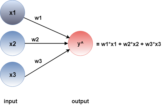
It is a graphical representation of a linear model represented with nodes and edges. It has three inputs x1, x2 and x3 with their associated weights w1, w2 and w3 respectively. There’s usually an additional bias term b to each of the inputs, however for simplicity let’s assume that there is no bias term in this model. The inputs and weights are mapped to output y ̂ which can be a class label (classification task) or a real-valued result (regression task). The output y ̂is calculated from the following formula,
y ̂ = w1*x1 + w2*x2 + w3*x3
Since it is calculating a linear formula, we can refer to this model as a linear model. Now, unfortunately in most of the cases real world data is hardly linearly separable. Therefore, we often need to add some non-linearity to our classification or regression model. Non-linearity adds new dimensions to the feature space which turns out helpful because linearly inseparable data often becomes separable when transformed to higher dimensions. To add non-linearity to this linear model let’s add an intermediate layer having three nodes or neurons between the input and output. This intermediate layer is called hidden layer.
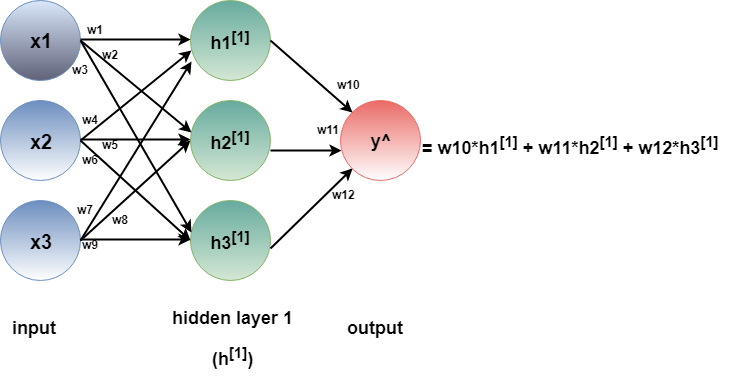
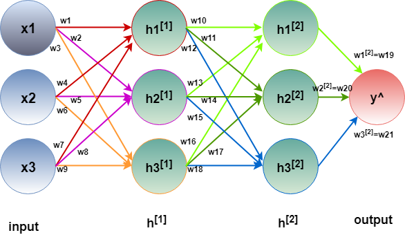
In figure 2, each input now has three edges towards each of the hidden nodes h1, h2 and h3 in hidden layer 1. This model can be labelled as a neural network, considering each hidden node as a neuron. The output y ̂ is now calculated by the following,
y ̂ = w10*h1[1] + w11*h2[1] + w12*h3[1]
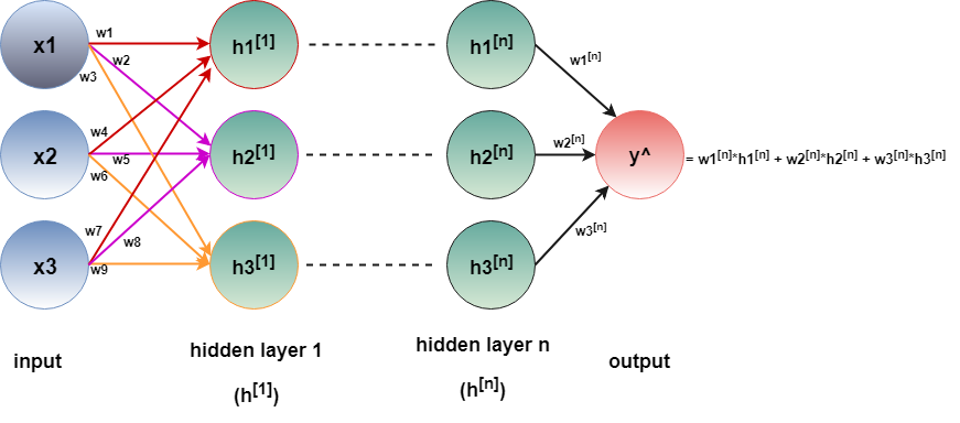
Theoretically, there can be as many intermediate hidden layers as possible. In figure 3, there are n number of hidden layers. The calculation carries on the same way like the model with a single hidden layer, although the number of parameters (i.e. weights) to compute increase exponentially.
Now, let’s go back to our initial question. How many hidden layers are needed to call a neural network a deep neural network? In other words, how deep is deep enough?
In order to answer this question, we need to understand the linear algebra taking place under the hood. In figure 4, each of the hidden nodes are calculated only from the edges coming towards them (incoming edges with same color).
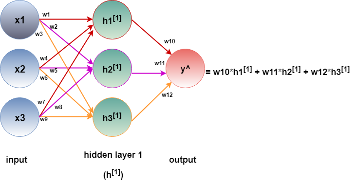
Therefore,
h1[1] = w1*x1 + w4*x2 + w7*x3
h2[1] = w2*x1 + w5*x2 + w8*x3
h3[1] = w3*x1 + w6*x2 + w9*x3
Combining all three, at the output node we have,
y ̂ = w10*h1[1] + w11*h2[1] + w12*h3[1]
However, h1, h2 and h3 are just linear combinations of input feature. Expanding the above equation, we end up having the following,
y ̂ = (w10*w1 + w11*w2 + w12*w3) *x1 + (w10*w4 + w11*w5 + w12*w6) *x2 + (w10*w7 + w11*w8 + w12*w9) *x3
It gives us a complex set of weight constants multiplied with original inputs. Substituting each group of weights with a new weight gives us the following,
y ̂ = W1*x1 + W2*x2 + W3*x3
which is exactly of the same form to our very first equation from the linear model! We can test this with as many number of hidden layers we want with a huge set of weights. However, after all the complex calculations, eventually our model will collapse into nothing but a linear model.
Let’s look at this from the algebraic perspective for the model in figure 5.
We are basically multiplying multiple matrices in a chain throughout the entire model. If we consider the first hidden layer as a vector H1 with three components h1[1], h2[1] and h2[1], represent all the weights between the input and H1 as a weight matrix W1 and x1, x2, x3 as input vector X, then we get the following,
H1 is a 3×1 vector obtained from 3×3 matrix W1 transposed multiplied by 3×1 input vector X. That’s how the values of the first hidden layer neurons are found. To find the second hidden layer neurons, we have to multiply the second layer weight matrix W2 transposed with the resultant matrix obtained from H1.
As we can see, two 3×3 matrices can be combined to a single 3×3 matrix by calculating their matrix products. This still gives the same shape for H2. We can test this with a different number of neurons in the second hidden layer. Let’s say instead of 3, H2 has two neurons. Therefore, the expected shape of H2 vector would be 2×1.
Thus, the shape of H2 still persists and the values for each of the neurons in H2 are rightly calculated. Now, let’s calculate the final output by adding the weight matrix consists of weights between the final layer (i.e. output) and H2. We assume that there are three neurons in H2.
Once again, our large chain of matrix multiplication has collapsed into a single 3-valued vector. In fact, if we train both the linear model and this 2-hidden layer neural net and stop at the same loss value, we will see that the weights learned by the linear model would exactly match with the weights learned by the latter, even after performing huge number of calculations. That means, just stacking up layers after layers in a network is not sufficient to add non-linearity to the model. As long as non-linearity is not added, the model is no better than a linear model, thus cannot be called as ‘deep’ no matter how many layers we have in between.
How to add non-linearity then? By adding a non-linear transformation layer which is facilitated by a non-linear activation function. In other words, in the computation graph in figure 6, we can imagine each hidden layer having two nodes in place of each single node.
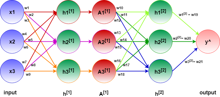
The green node is calculating the input coming through the incoming edges, which is a linear function. The output to this node is then passed to the next red node which transforms that linear equation to a non-linear one. Finally, the output of the red node is then passed to the next hidden layer. So, the activation acts as the transition point between two hidden layers. Adding this non-linear transition point is the only way to stop a neural network condensing back to a shallow linear model. There are many activation functions for this transformation like sigmoid, tanh, ReLu etc. Even if we have an activation function between two intermediate layers and don’t have them somewhere else, then those consecutive layers will collapse to a single layer due to the same principal discussed above. For this same reason, we see that most neural networks have activation functions (mostly ReLu) between all the hidden layers and linear for regression and sigmoid or softmax function for classification before the final output.
Let’s compare this new network in figure 6 to the previous network in figure 5 from linear algebra perspective. For an activation function, we add ReLu between H1 and H2. For each of the component in the resultant matrix of W1TX, ReLu will take the maximum of zero and that component. In other words, in the positive domain, the original value retains however in the negative domain we set the value as zero. Because this activation function is applied element-wise to the resultant matrix, there is no way to express f(W1TX) in terms of a matrix in linear algebra. Thus, that portion of the transformation chain can be collapsed into a simpler or linear function. As a result, the complexity of the network remains and does not get simplified into a linear combination of inputs.
However, the final layer and hidden layer 2 or H2 can still be transformed to a linear function because there is no non-linearity added in between.
Therefore, the answer to our initial question is, to consider a neural network as a deep neural network, there must be some kind of non-linearity or complexity being passed between the layers in hierarchical order (i.e. output of hidden layer activation function is passed as input to the next hidden layer). With complexity being pertained, neural network with a single hidden layer can be considered as ‘deep’ whereas without complexity layers after layers stacked to the network will not be enough to make it a ‘deep neural net’.
I hope you have found this article useful. Please feel free to comment below about any questions, concerns or doubts you have. Also, your feedback on how to improve this blog and its contents will be highly appreciated. I would really appreciate you could cite this website should you like to reproduce or distribute this article in whole or part in any form.
You can learn of new articles and scripts published on this site by subscribing to this RSS feed.
Hello, I find your writing very insightful.
Thank you!